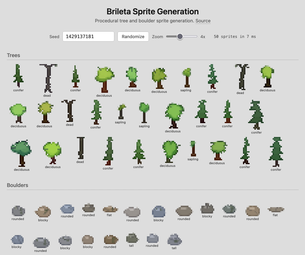
Brileta is a game engine and roguelike sandbox I’ve been building as a hobby project. You can try the sprite generator live in your browser.
It started as me playing around with roguelike mechanics - turn-based movement on a tile grid, field of view, pathfinding - and I kept thinking that I’d eventually switch to a proper engine. Instead, I kept adding things. Lighting with ray-marched shadows. Procedural world generation. Rain and weather effects. At some point I looked up and realized I’d built an engine.
I thought it would be fun to write up how different parts of it work, starting with the procedural sprite system.
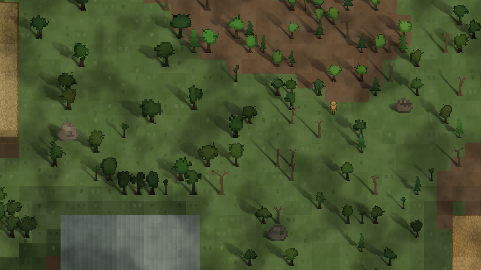
Everything in a Brileta world is generated from a single seed, including the sprites. Every tree and every boulder is unique, generated once, never stored. A deciduous oak on one tile has a different canopy than the one three tiles over. A granite slab near the road has lichen that the cracked sandstone wedge beside it doesn’t.
On a single core of an M4 MacBook Pro, the Python/C engine generates 300 tree sprites and 80 boulder sprites for a typical map in about 16ms - less than one frame at 60fps. And it only needs to happen once at map generation.
This post walks through the system that produces them.
One Seed, One Sprite
Every sprite starts with a spatial seed - a deterministic hash of the object’s world position and the map’s master seed:
def derive_spatial_seed(x, y, *, map_seed, salt=0):
    return (
        (x * 73856093)
        ^ (y * 19349663)
        ^ map_seed
        ^ salt
    ) & 0xFFFFFFFF
The same position on the same map always gives you the same sprite. Different salt values give independent random streams for different properties (the sprite itself vs. its height jitter, for example), so changing one doesn’t cascade into the other.
From this seed, all downstream randomness flows through a seeded xoshiro128++ PRNG (initialized via SplitMix64). Why not Python’s built-in random module? Two reasons: it’s too heavy for the C inner loop where sprites are rasterized, and it needed to be deterministic across both the Python engine and the TypeScript port. The same seed should produce the same sprite on every platform.
The result of all this is that the game can regenerate any sprite on demand without storing it. Revisit a corner of the map, and that one weird conifer with the leftward lean is exactly where you left it.
The Sprite Rendering Toolkit
Trees and boulders look very different, but they’re built from the same set of drawing primitives.
Soft Ellipses
The core primitive is a soft ellipse - fully opaque in the center and fading to transparent at the edges.
Two parameters determine what the ellipse looks like: falloff and hardness.
Hardness determines how much of the ellipse is fully solid. At hardness 0, only a small core is fully opaque and most of the ellipse is soft fade. At hardness 1, nearly the entire ellipse is solid with just a thin fringe at the edge.

Falloff controls the shape of that fade. A falloff below 1.0 makes opacity drop quickly - you get a crisp edge. Above 1.0, opacity stays high through most of the fade zone before dropping at the outer edge - you get a puffy, cloud-like shape.

A single deciduous tree can have 30+ overlapping ellipses across its three tone passes. Standard alpha compositing is order-dependent - drawing ellipse A then B gives a different result than B then A. When you batch dozens of ellipses per tree, that’s fragile.
Instead, ellipses accumulate into a float32 opacity buffer using an order-independent formula: 1 - product(1 - alpha_i). Each ellipse contributes its alpha, and the result is the same regardless of draw order.
The full precision survives until the final step converts to 8-bit color. At 20 pixels, rounding artifacts are visible, so the extra precision matters.
Three-Tone Shading
Both trees and boulders use three color tones stamped in separate passes: shadow, mid, highlight. The system derives these from a base color by shifting each RGB channel:
mid = base
shadow = shift_color(base, -55, -50, -30)
highlight = shift_color(base,  55,  45,  20)
Those shifts are huge - on a 0-255 scale, the shadow and highlight are over 100 points apart per channel. At full resolution, this could look garish, but at 16-20 pixels it’s just right. Subtlety doesn’t survive miniaturization.
The three passes use different ellipse parameters to create directional lighting:
| Pass | Falloff | Hardness | Placement |
|---|---|---|---|
| Shadow | 1.8 | 0.80 | Lower, wider |
| Mid-tone | 1.5 | 0.70 | Centered |
| Highlight | 1.3 | 0.60 | Upper, smaller, softer |
Shadows anchor the base with hard edges. Highlights float near the top with soft falloff. The mid-tone bridges them. Together, the three passes create a convincing sense of volume from flat ellipse stamps.
After all three passes, a rim darkening step finds every pixel adjacent to transparency and subtracts 30 from each RGB channel. This thin dark outline sharpens the silhouette against any background without requiring a separate outline layer.
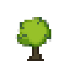
Growing a Deciduous Tree
Deciduous trees are where most of the geometric complexity lives and where the toolkit gets the hardest workout. On a typical 20x20 pixel canvas (with ±3 pixels of size jitter per instance), here’s how they come together.
Rather than stamping one big green oval, the system places 3-6 lobes in a ring around the canopy center, then fills each lobe with overlapping ellipses across the three tone passes.
Lobes are spaced evenly around the canopy center like hours on a clock face, then jittered by a random angle so they don’t look regular. Each lobe sits about halfway between the center and the canopy edge. The vertical axis is compressed below the center, which pushes the canopy mass upward and gives it a natural crown shape rather than a perfect circle.
Each lobe gets its own set of shadow, mid, and highlight ellipses - 1-3 per tone, per lobe. A few central fill ellipses bridge the gaps between lobes so the canopy reads as one continuous mass rather than a cluster of disconnected blobs.
After the canopy, 2-5 branch tip extensions - short line segments poking outward from lobe edges - break up the smooth elliptical contour. These are small, but at this scale they make the difference between “oval” and “tree.”
The trunk tapers from a wide base to where it meets the canopy, with a slight random lean of up to 1.5 pixels. Some trunks get a root flare at the bottom. Four trunk color palettes (warm browns) with slight color variation ensure no two trunks match.
There are also crown shape variants. About 35% of deciduous trees get the default round crown, 20% get a narrow-tall crown, 30% get a wide-squat crown, and the remaining 15% get a round crown offset horizontally from the trunk. These stacked variations on top of the per-lobe randomness are what make each deciduous tree visually distinct.
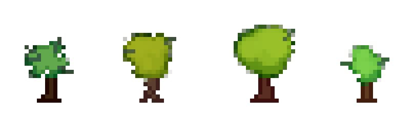
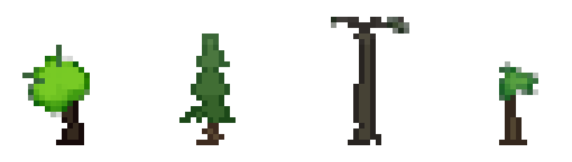
The Other Tree Archetypes
Conifers skip the lobe system entirely. They stack 3-6 filled triangles, each narrower than the one below, with ~35% vertical overlap. Each tier gets progressively lighter from base to crown. The tier widths and positions accumulate small per-tier offsets, so the silhouette isn’t perfectly symmetric. The result reads as a classic conifer triangle at a distance, but up close each one has a slightly different tier count, lean, and color progression.
Dead trees are skeletons. Same trunk as deciduous, but the branches split into two at each level - 4 levels deep instead of 2 - with wider angular spread and more asymmetry between left and right forks. No canopy fill - just the branches themselves, visible against sky. A few moss or lichen spots at branch junctions add a touch of color to the otherwise monochrome silhouette.
Saplings are miniature deciduous trees - 2-4 lobes instead of 3-6, on a smaller canvas (10-18 pixels). The color shifts between shadow and highlight are gentler, giving them a softer look that reads as younger growth.
Forest Zoning
Scattering all four archetypes uniformly would look wrong - real forests have zones. Brileta uses OpenSimplex noise to create species gradients across the map.
The 75% living share is split between deciduous and conifer based on a noise field sampled at each tree’s position. Where noise is high, conifers dominate (~92% of living trees). Where it’s low, deciduous trees take over. The transition zones create natural-looking mixed forest. Dead trees and saplings scatter uniformly regardless.
The noise field layers multiple octaves of simplex noise via fractional Brownian motion (FBM), so you can tune cluster size and boundary sharpness by adjusting octave weights without touching the generation code.
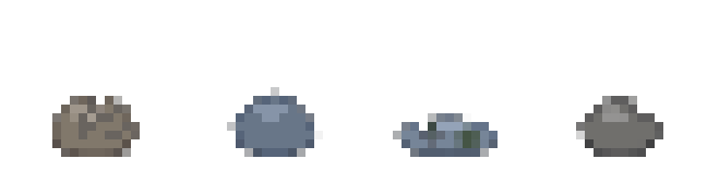
Boulders
Where trees grow upward from a trunk, boulders cluster ellipses into low, heavy horizontal masses. They use the same three-tone shading but with tighter color shifts, since stone is lower-contrast than foliage.
Four archetypes, each a different way of arranging the ellipse clusters:
- Rounded (35%) - wide, low profile with a few side bumps
- Tall (20%) - portrait aspect ratio, wide base tapering to a narrow crown
- Flat (25%) - a low slab, wider than it is tall
- Blocky (20%) - the ellipses cluster to one side instead of spreading evenly, creating a lopsided mass with crisper edges
Boulder colors pull from 11 stone tones with slight brightness and warm/cool variation per instance, ranging from pale sandstone to dark granite.
What makes boulders interesting is the surface detail. After the base shape is stamped, two passes add character:
Cracks appear on ~60% of boulders. Each is a short line (1.5-3.5 pixels) starting from the upper surface and running inward, drawn darker than the shadow tone. 1-3 per boulder, with random angles biased downward from the top face.
Lichen appears on ~50% of boulders. Each spot is a tiny soft ellipse (radius 0.7-1.5px) in muted green or yellow at low opacity, placed on the upper face of the boulder. The low hardness (0.15) makes them blend into the stone surface rather than sitting on top of it.
Breaking the Silhouette
After everything else, both trees and boulders go through a nibbling pass that randomly removes edge pixels.
The system finds every edge pixel - any opaque pixel next to transparency - and randomly decides whether to erase it. Trees nibble in two phases. First, each edge pixel has a ~25% chance of being erased. Then a second pass carves inward from each removed pixel toward the center at ~10% probability, creating small notches rather than just single-pixel holes.
Boulders nibble more gently (~10-14% probability) and only on the upper half of the shape. The bottom edge stays solid - a boulder sitting on the ground shouldn’t have gaps at its base.
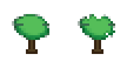
Without nibbling, every canopy is a smooth ellipse cluster and every boulder is a tidy ellipse stack - technically correct, but lifeless. It was the change that made me stop seeing caricatures and start seeing truly organic shapes.
Performance
Sprite generation is pure CPU rasterization. At 20x20 pixels per canvas, even the most complex tree only writes to a few hundred pixels per pass.
The Python/C engine generates 300 trees and 80 boulders for a typical map in about 16ms on a single core of an M4 MacBook Pro. The TypeScript port that powers the live demo generates 50 sprites in about 6ms - slower per sprite than the C path, but more than fast enough for interactive use.
What Else Could You Draw?
Trees and boulders share about 70% of their code, and nothing here is specific to organic shapes. Soft ellipses with tunable hardness, three-tone shading, edge nibbling - the same primitives could generate bushes, mushrooms, flower patches, whatever your world needs.
The brileta-sprites TypeScript library is MIT-licensed. If you try it in your own project, show me what you make.